Computing in the Big Data Cluster with PySpark using Jupyter Notebooks
- Introduction
- Use Lmod to load the required software
- Specify PySpark configuration
- Launch the PySpark job
- A simple demonstration of PySpark
Introduction
Jupyter notebooks
are a popular way of executing code with an in-browser GUI. In addtition
to code execution, they support plotting, markdown, and much more functionality
with the aim of tightly integrating code and documenation. The simplest
way to view a Jupyter notebook running remotely is to use port forwarding via ssh,
for example:
ssh -L 9999:<remote_host>:8889 <remote_host>
This will forward the notebook running on the remote host at port 8889 to your local port 9999.
To see what’s happening on your local port 9999, just type localhost:9999 into the address
bar of your favorite browser. Since we haven’t started the notebook, you shouldn’t see anything yet.
Use Lmod to load the required software
The Big Data cluster now uses Lmod to load software packages, just like the main ACCRE cluster. The Big Data cluster has its own set of packages specific to big data workflows, including Spark. So, the first step in getting our Jupyter notebook up and running is to load Spark and Anaconda
ml purge
ml Spark/2.2.0 Anaconda3/4.2.0
Specify PySpark configuration
The module Anaconda3 contains the pertinent commands that we need to run PySpark,
namely python3 and jupyter. To use these commands, we need to tell Spark
which version of Python we need to use; this happens in a few places.
Spark executors are launched on the worker nodes in the cluster, and the
PYSPARK_PYTHON environemnt variable tells Spark workers which version of Python to use.
export PYSPARK_PYTHON=$(which python3)
This works because all Lmod software is installed in the /opt directory,
an NFS mounted directory that is shared across
the entire big data cluster. So even though Lmod is only installed on the gateway node,
the python3 command is present on each machine in the cluster at the path returned
by $(which python3).
For PySpark applications, the Spark driver should execute on the client node. In this
case, we need to tell the driver to execute the jupyter command rather than a python
command:
export PYSPARK_DRIVER_PYTHON=jupyter
export PYSPARK_DRIVER_PYTHON_OPTS="notebook --no-browser --port=8889 --ip="*""
Setting PYSPARK_DRIVER_PYTHON to jupyter is, admittedly, a bit of a hack, since jupyter
doesn’t actually function the same way as python. As you may have already guessed,
PYSPARK_DRIVER_PYTHON_OPTS specifies everything passed to the jupyter command.
Launch the PySpark job
The Spark/2.2.0 module makes available the pyspark command, which is what we’ll use to
kick off our interactive job:
pyspark --master yarn
The --master yarn option tells PySpark that we want to use YARN to schedule our job across
the Big Data cluster; if we omitted it, we would simply run PySpark on the gateway node
without access to the HDFS filesystem and the computational power of the worker nodes. Thus,
this is usually what you want, unless you’re doing small testing or debugging. The magic of
distributing your job across the cluster with this single option is made possible by the
environment variable HADOOP_CONF_DIR which is automatically set when you load Spark/2.2.0.
After running the above command, you should see some normal logging output from the
jupyter notebook command, so now log in to localhost:9999 and you should see the
Jupyter file browser launched from your directory on the cluster.
Click on New > Python [default] and Voila! You now have a new Jupyter notebook instance.
A simple demonstration of PySpark
The content in this section comes from the pyspark-notebook-example in our GitHub repo.
Pro Tip: The command jupyter nbconvert --to markdown <notebook>.ipynb converts
a Jupyter notebook to pure markdown, making it easy to incorporate into blog posts, for example!
%matplotlib inline
import matplotlib.pyplot as plt

import pyspark
import random
import time
Estimate \(\pi\)
As a simple example, let’s approximate \(pi\) with brute force.
Define a function to decide whether a randomly chosen point in the \(XY\) plane lies inside the unit circle.
def inside(p):
    x, y = random.random(), random.random()
    return x*x + y*y < 1
Define a function that uses the SparkContext, sc, to distribute the work across partitions
def approx_pi(num_samples, num_partitions):
    num_inside = sc.parallelize(range(0, num_samples), num_partitions).filter(inside).count()
    pi = 4 * num_inside / num_samples
    return pi
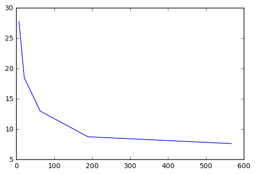
Explore how the number of partitions affects the speed of the computation.
samples = 100000000
num_partitions = 7
errors = []
times = []
partitions = []

for _ in range(5):
    t0 = time.time()
    pi_approx = approx_pi(samples, num_partitions)
    t1 = time.time()


    dt = t1 - t0
    errors.append(pi_approx - 3.1415926536)
    times.append(dt)

    partitions.append(num_partitions)
    num_partitions *= 3


plt.plot(partitions, times)
[<matplotlib.lines.Line2D at 0x7f59449b80f0>]
Test for Benford’s law
Let’s count the occurence of numeric digits within a body of text and decide if the distribution of digits follows Benford’s law. The data we’ll explore are bikeshare records in DC, currently available in the shared /data directory on the Big Data cluster. For example:
$ hadoop fs -cat /data/capitalbikeshare-data/2016-Q3-Trips-History-Data-1.csv | head -20
Duration (ms),Start date,End date,Start station number,Start station,End station number,End station,Bike number,Member Type
840866,8/31/2016 23:59,9/1/2016 0:13,31117,15th & Euclid St  NW,31228,8th & H St NW,W20409,Registered
656098,8/31/2016 23:58,9/1/2016 0:09,31279,19th & G St NW,31600,5th & K St NW,W20756,Registered
353159,8/31/2016 23:58,9/1/2016 0:04,31107,Lamont & Mt Pleasant NW,31101,14th & V St NW,W22626,Registered
219234,8/31/2016 23:58,9/1/2016 0:02,31200,Massachusetts Ave & Dupont Circle NW,31212,21st & M St NW,W00980,Casual
213473,8/31/2016 23:56,8/31/2016 23:59,31281,8th & O St NW,31280,11th & S St NW,W21338,Registered
637695,8/31/2016 23:56,9/1/2016 0:07,31624,North Capitol St & F St NW,31241,Thomas Circle,W21422,Registered
356455,8/31/2016 23:54,9/1/2016 0:00,31034,N Randolph St & Fairfax Dr,31023,Fairfax Dr & Wilson Blvd,W00748,Casual
924793,8/31/2016 23:53,9/1/2016 0:08,31124,14th & Irving St NW,31267,17th St & Massachusetts Ave NW,W21480,Registered
309433,8/31/2016 23:53,8/31/2016 23:58,31242,18th St & Pennsylvania Ave NW,31285,22nd & P ST NW,W20113,Registered
447572,8/31/2016 23:52,8/31/2016 23:59,31007,Crystal City Metro / 18th & Bell St,31011,23rd & Crystal Dr,W00943,Registered
438823,8/31/2016 23:52,8/31/2016 23:59,31122,16th & Irving St NW,31214,17th & Corcoran St NW,W00833,Registered
350341,8/31/2016 23:51,8/31/2016 23:57,31264,6th St & Indiana Ave NW,31244,4th & E St SW,W20404,Registered
568722,8/31/2016 23:51,9/1/2016 0:01,31238,14th & G St NW,31201,15th & P St NW,W22750,Registered
229685,8/31/2016 23:50,8/31/2016 23:54,31304,36th & Calvert St NW / Glover Park,31226,34th St & Wisconsin Ave NW,W21185,Registered
405098,8/31/2016 23:50,8/31/2016 23:57,31212,21st & M St NW,31114,18th St & Wyoming Ave NW,W22401,Registered
2592652,8/31/2016 23:47,9/1/2016 0:30,31067,Columbia Pike & S Walter Reed Dr,31260,23rd & E St NW ,W21736,Registered
570531,8/31/2016 23:46,8/31/2016 23:56,31111,10th & U St NW,31122,16th & Irving St NW,W21005,Registered
981529,8/31/2016 23:46,9/1/2016 0:03,31235,19th St & Constitution Ave NW,31258,Lincoln Memorial,W22953,Registered
1138485,8/31/2016 23:45,9/1/2016 0:04,31000,Eads St & 15th St S,31000,Eads St & 15th St S,W21251,Casual
Define our mapping function that will count the number of digits
def count_digits(string):
    counter = [0] * 10
    for c in string:
        if c in '0123456789':
            counter[int(c)] += 1
    return counter

dummy_counter = count_digits('abcd111123234')
print(dummy_counter)
[0, 4, 2, 2, 1, 0, 0, 0, 0, 0]
Define a reduce function that combines two counters into one.
def combine_digits(a, b):
    # assert(len(a) == len(b) == 10)
    return [a[i] + b[i] for i in range(10)]

print(combine_digits(dummy_counter, dummy_counter))
[0, 8, 4, 4, 2, 0, 0, 0, 0, 0]
Apply the map and reduce functions
lines = sc.textFile('/data/capital*/*.csv', 60) # notice the globbing functionality in the file names
counts = lines.map(count_digits).reduce(combine_digits)
print(counts)
[89309440, 133682530, 96328002, 50280321, 38989407, 37620303, 30666030, 27789765, 26541711, 23779326]
Plot the counts as a histogram.
fig, ax = plt.subplots()
ax.bar(range(1,10), counts[1:], align='center')
ax.set_ylabel('Counts')
ax.set_xlabel('Digit')
ax.set_xlim(0.5, 9.5)
ax.set_xticks(range(1, 10))
# ax.set_xticklabels(range(1,10))
[<matplotlib.axis.XTick at 0x7f5946d62908>,
 <matplotlib.axis.XTick at 0x7f5944399550>,
 <matplotlib.axis.XTick at 0x7f59443a5e48>,
 <matplotlib.axis.XTick at 0x7f5944935f98>,
 <matplotlib.axis.XTick at 0x7f594493a9e8>,
 <matplotlib.axis.XTick at 0x7f594493c438>,
 <matplotlib.axis.XTick at 0x7f594493ce48>,
 <matplotlib.axis.XTick at 0x7f5944940898>,
 <matplotlib.axis.XTick at 0x7f59449442e8>]
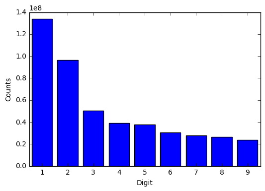
A set of numbers is said to satisfy Benford’s law if the leading digit \(d (d ∈ {1, …, 9})\) occurs with probability
from math import log10

total_counts = sum(counts[1:])
probs = [cts / total_counts for cts in counts]

for d, prob in enumerate(probs):
    if d == 0:
        continue
    ideal = log10(1 + 1 / d)
    print("Ideal: {0} --- Actual {1}".format(ideal, prob))
Ideal: 0.3010299956639812 --- Actual 0.28707111711961025
Ideal: 0.17609125905568124 --- Actual 0.20685565379440418
Ideal: 0.12493873660829992 --- Actual 0.10797243228866628
Ideal: 0.09691001300805642 --- Actual 0.08372621780363636
Ideal: 0.07918124604762482 --- Actual 0.08078619104970727
Ideal: 0.06694678963061322 --- Actual 0.06585252006917794
Ideal: 0.05799194697768673 --- Actual 0.05967600166634672
Ideal: 0.05115252244738129 --- Actual 0.05699591881628697
Ideal: 0.04575749056067514 --- Actual 0.05106394739216406